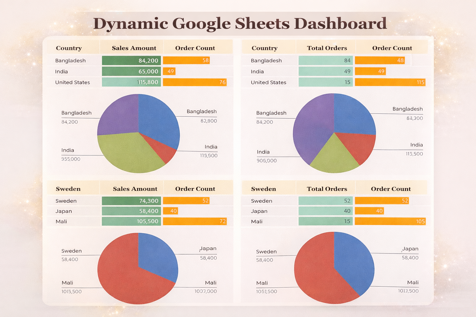
Create Dynamic Pivot Charts from Pivot Tables
Dynamic pivot charts allow you to turn static spreadsheet data into interactive, filterable visuals that update instantly. Instead of rebuilding charts manually, pivot charts connected to pivot tables respond automatically to slicers and selections.
In this guide, we’ll create dynamic pivot charts from pivot tables step by step using Excel’s built-in tools - no formulas required. We’ll start with the easiest method pure pivot charts.
Download and Open the Practice File
- Download the Dynamic Charts – Empty File from Additional Resources
- Open the file in Excel
- Navigate to the sheet named Built Regular
This sheet already contains correctly structured data, so you can focus on chart creation instead of cleanup.
Select the Data Range
- Select the entire dataset
- Ensure headers (Business Units, Years, Sales) are included
Proper selection ensures Excel builds the pivot table correctly.
Insert a Pivot Chart

- Go to Insert → PivotChart
- Choose PivotChart
- Select New Worksheet
- Click OK
Excel automatically creates:
- A pivot table
- A pivot chart linked to that table
Configure Pivot Chart Fields
Set the following:
- Axis (Categories): Years
- Values: Sales
- Legend (Series): Business Units
Resize the chart slightly once done.
Remove Field Buttons
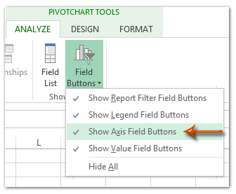
- Right-click any field button on the chart
- Select Hide All Field Buttons on Chart
This removes visual clutter.
Adjust Legend Position
- Move the legend to the bottom for better readability.
Remove Axis and Gridlines
- Delete axes
- Delete gridlines
This creates a clean dashboard-style visual.
Add Data Labels
- Enable data labels
- Optional: make labels bold
Values are now readable without axes.
Remove Chart Outline
- Set Outline → No Outline
Remove Background Gridlines
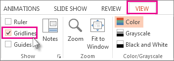
- Press Ctrl + A
- Go to View
- Uncheck Gridlines
Insert Slicers
- Go to PivotChart Analyze → Insert Slicer
- Select:
- Years
- Business Units
Slicers make the chart fully interactive.
Resize and Style Slicers
- Resize slicers to show multiple items
- Adjust colors if needed
- Place slicers beside the chart
Filter by Business Unit
Click any business unit (e.g., Dentist).
The chart updates instantly.
Filter by Multiple Years
- Hold Ctrl
- Select multiple years
The pivot chart recalculates automatically.
Why This Method Works
- Fast to build
- No formulas required
- Fully interactive
- Ideal for dashboards and reports
- Updates automatically with new data
Practice Recommendation
Repeat this process using the practice file:
- Test stacked or bar pivot charts
- Try different slicer combinations
- Experiment with formatting styles
Want This Fully Automated?
VizMint applies these exact concepts automatically by converting Excel files into interactive dashboards — no pivot setup required.