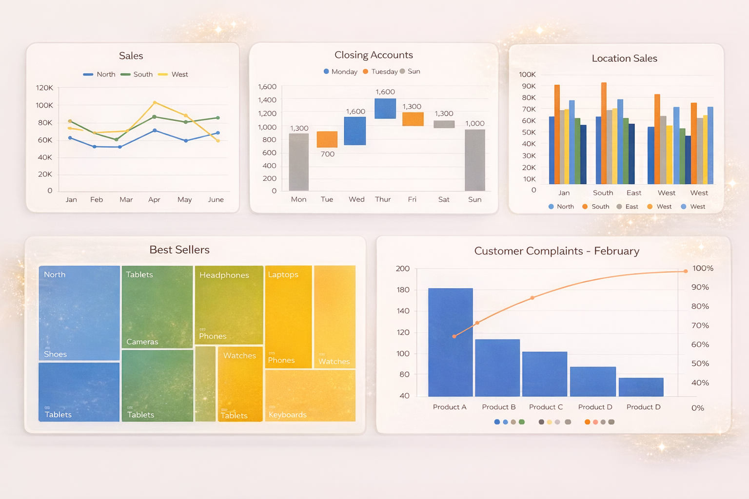
Turn Excel Data Into a Graph
If you’ve ever stared at a spreadsheet full of numbers and thought, “There has to be a better way to understand this,” you’re absolutely right.
Today, we’re going to learn how to turn Excel data into a graph, specifically bar charts and column charts, using Microsoft Excel. We’ll also cover multi-column charts and stacked column charts, so you know exactly which chart to use and when.
By the end of this guide, you’ll be able to transform raw Excel data into clear, visual insights—no guesswork required.
Why Turn Excel Data Into a Graph?
Tables are great for storing data, but charts are better for understanding it.
Graphs help you:
- Compare values instantly
- Spot trends and patterns
- Explain data clearly to others
- Make faster, more confident decisions
Instead of scanning rows and columns, a chart lets your brain do the work visually.
Example Data: Sales Table in Excel
Let’s say you have a simple Excel table with sales data, such as monthly sales for different products.
You could try to analyze this by reading the numbers, but a graph makes insights obvious. That’s where bar charts and column charts come in.
How to Turn Excel Data Into a Column Chart
A column chart displays data using vertical bars, making it ideal for comparing values across categories or over time.
Step-by-step:
1. Open your Excel worksheet
2. Click anywhere inside your data table
3. Go to the Insert tab at the top
4. In the Charts section, click the Column Chart icon
5. Choose a basic 2D Column Chart
Excel will instantly insert a column chart onto your worksheet, allowing you to see which values are higher, lower, or trending upward.
Bar Chart vs Column Chart (What’s the Difference?)
Understanding this difference helps you choose the right graph.
Column Chart
- Vertical bars
- Best for time-based data (months, years)
- Easy comparison across categories
Bar Chart
- Horizontal bars
- Best when category names are long
- Works well with many data points
Both display the same information—just in different orientations.
How to Create a Bar Chart in Excel
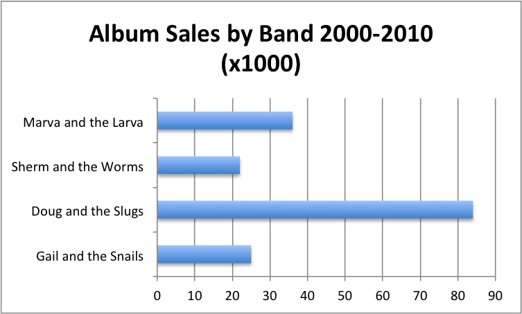
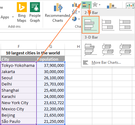
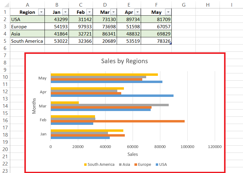
To switch from a column chart to a bar chart:
1. Select your data
2. Go to Insert → Bar Chart
3. Choose a 2D Bar Chart
Your data will now appear horizontally, which can be easier to read when labels are long.
Making a Multi-Column Chart
A multi-column chart lets you compare multiple values side by side.
Examples include:
- Product A vs Product B
- This year vs last year
If your Excel data contains multiple columns, Excel automatically groups the bars or columns for comparison.
How to Create a Stacked Column Chart

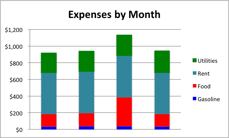 A stacked column chart shows the total value while also showing how each part contributes to that total.
Use stacked charts when:
- You want to show composition
- You are analyzing proportions
- You need totals and breakdowns together
To create one:
1. Select your data
2. Go to Insert → Column Chart
3. Choose Stacked Column
Customizing Your Excel Graph
Once your chart is inserted, you can:
- Change colors
- Add chart titles
- Edit axis labels
- Switch chart types
Excel offers flexibility, but customization still takes time.
A Faster Way to Turn Excel Data Into a Graph
Excel works well, but it’s still manual.
If you want to turn Excel data into graphs instantly—without choosing chart types or adjusting layouts—VizMint can help.
With VizMint, you can:
- Upload an Excel or CSV file
- Automatically generate clean charts
- Instantly visualize trends and insights
- Skip manual formatting entirely
It’s built for people who want answers, not chart setup.
Final Thoughts
Learning how to turn Excel data into a graph is a foundational skill, whether you’re analyzing sales, tracking performance, or presenting insights.
- Use column charts for vertical comparisons
- Use bar charts for horizontal clarity
- Use stacked charts to show composition
And when you’re ready to move faster than Excel alone, VizMint turns spreadsheets into insights automatically.